Annoy algorithm
The Annoy algorithm is an algorithm used to approximate the nearest neighbors of a certain point. Annoy is built by partitioning the data into two halves, similar to a binary search tree. The annoy algorithm doesn’t guarantee the correct answer, but it gets super close at a fraction of the cost.
In Euclidean space, the distance between any two points can be determined by using the distance formula, which is derived from the Pythagorean theorem. The nearest neighbors to a point are the points where that distance is minimized.
The Naive Algorithm:
First, it’s important to talk about the naive algorithm used to calculate the K-nearest neighbors. Let’s say you’re given a scenario like the following: You wish to find the three closest black points to the blue point.
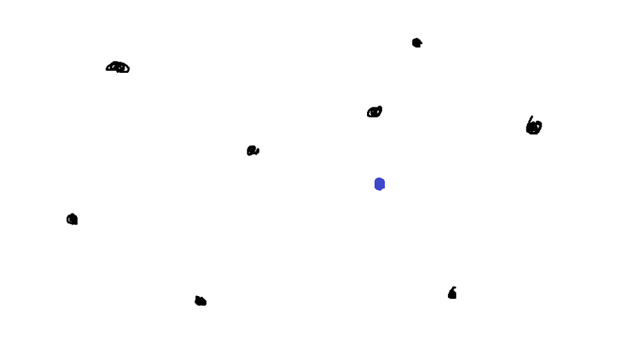
Everyone’s initial idea is to simply loop through all of the black points, calculating their distances to the blue point as they go. However, this operates in linear time, which is not ideal. The annoy algorithm is able to log n.
The Annoy Algorithm:
While creating the data structure to allow the approximation of nearest neighbors, the space is always cut in half. This algorithm for construction works recursively until it reaches a certain threshold. Initially, it picks two random points and creates a line, which splits the space into a part that lies above the line and a part that lies below the line.
Assume I chose to create this line using points 3 and 5.
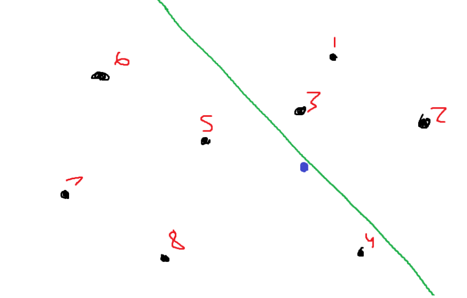
You can see that points 1, 2, and 3 all lie above the line. Points 4, 5, 6, 7, and 8 all lie below the line.
Specifics about creating the line:
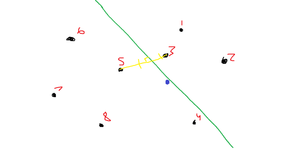
The green line is the perpendicular bisector of the straight line, which connects points 3 and 5. Refer to the following image with markings:
After we add this information to a binary tree, The right child will always hold the nodes that lie above the line, and the left child will always hold the nodes that lie below the line.
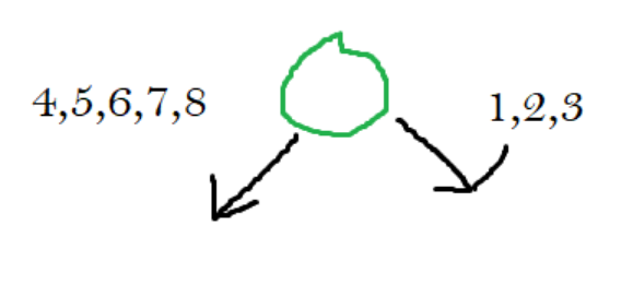
Then, we do this process of partitioning again on one of the children. In the first step, we cut the space into two halves. Our algorithm is recursive, and now we are going to break one of those halves into more halves.
Let’s say that I randomly chose points 5 and 8 to partition. I will get the following image now:
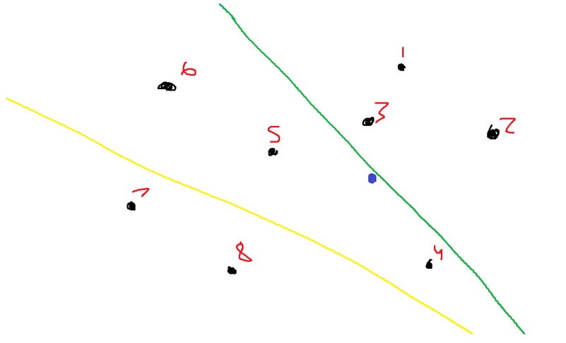
Then, I make sure to add this new information to the tree.
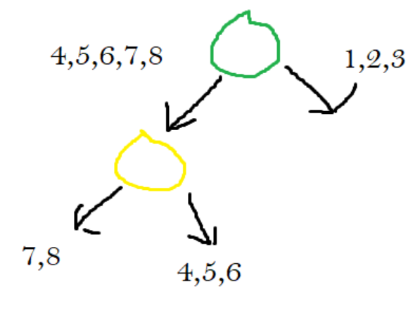
This concept of splitting the tree happens until a certain predetermined threshold. The programmer will set the maximum number of points that can be in each section. The leaf nodes are associated with the points that can be found in that section.
From the information supplied by the tree, we can conclude the following:
Points 1, 2, and 3 can be found by going above the green line.
Points 7 and 8 can be found by going below the green line and below the yellow line.
Points 4,5,6 can be found by going below the green line but above the yellow line.
However, let’s set that value to two. According to the algorithm, we must continue partitioning.
Let’s say in this iteration I chose points 4 and 5. Here is the new drawing.
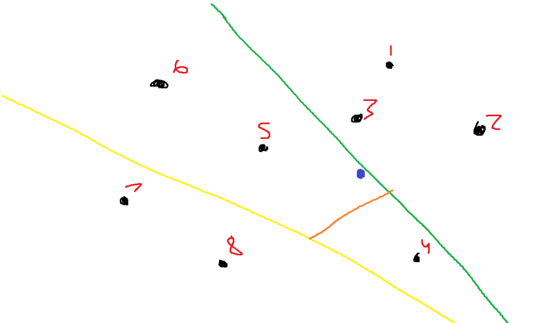
Our tree now looks like the following:
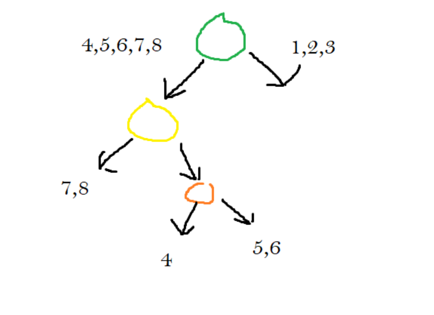
In the next iteration, I chose to use points 1 and 2. Our new space looks like the following:
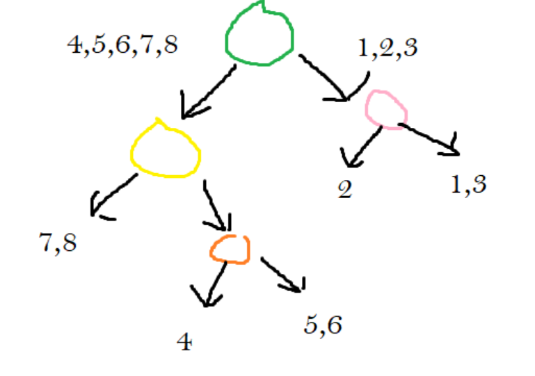
We notice that each section has two or fewer points. So, our algorithm will terminate.
Querying the closest neighbors:
For the following example, I’m using the image that was developed through this article. We are attempting to figure out the closest neighbors to the blue point.
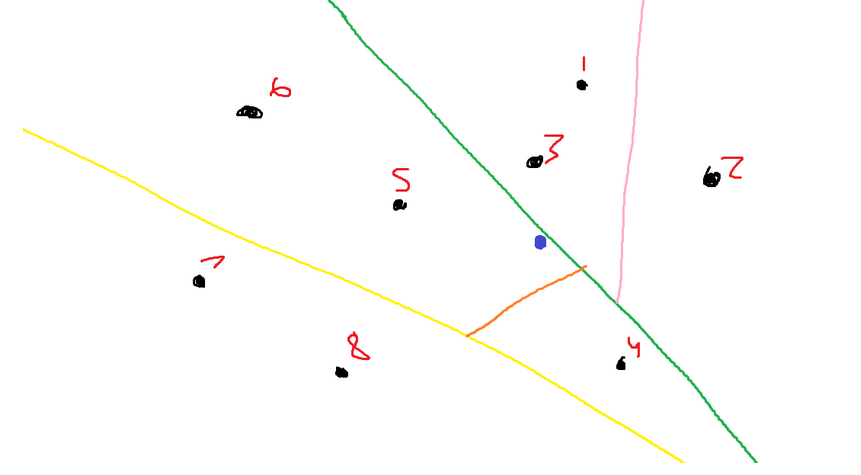
To find the closest neighbors to the blue point, we will start at the root node of our tree. The root node of our tree represents the green line. We will compare our blue point to the green line. Our point is below the green line, which means we continued on the left side of the tree.
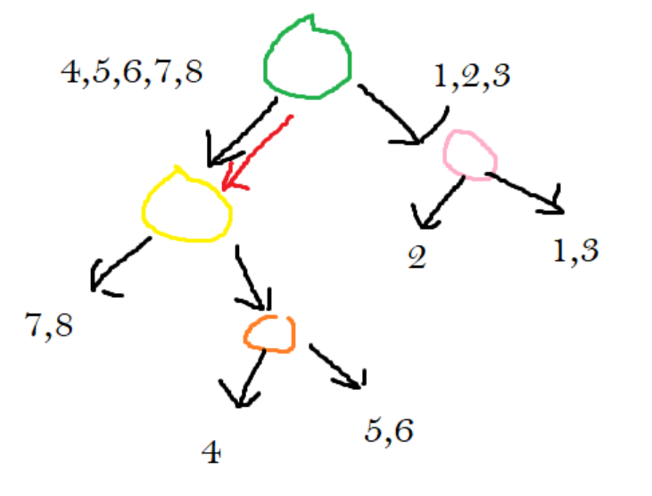
Now we are on the node that represents the yellow line. We need to figure out the blue points relative to the blue point. We figure out that the blue point lies above the yellow line, so we continue on its right.
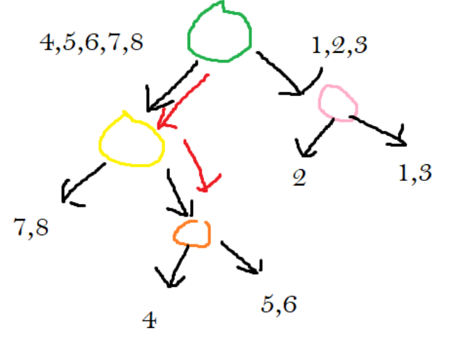
Now we are at the node that corresponds with the orange line. We figure out that the point lies above the orange line, so we traverse to its right child.
Once it went to its right child, we figured out that it was at a leaf node. It states that the points located in this section are points 5 and 6. These two points are what we will use as the answer to the nearest neighbor problem.
As you may have noticed, this answer is not even close to right. Throughout the process, the algorithm was picking random points to split the space by. Had the algorithm chosen better points, our answers might have been so poor.
Which might lead people to run this algorithm multiple times. I am hoping that they will come across a better way to cut up the space. They might test each partition against testing data and record the trees with the best performances. Getting a good partition is complete luck, but there is a value that programmers do have control over. This is the threshold value. In our problem, we decided that it was best to cut it off at two. This meant that no section had more than two points. Altering this threshold value might improve and is worth considering when finding the best cut.