Standard Deviation and Variance
The standard deviation and variance are both measures of how dispersed the data points are. The bigger the standard deviation or variance, the farther the data points are from the mean. A low variance means all of the points are packed closely to the mean. If all points lie on the mean, then there isn’t any variance.
Standard deviation and variance are closely related. As you will see later, variance is just the standard deviation squared.
The standard deviation describes how much spread there is from the mean of the data.
The variance describes the average of the squared distances of the data points from the mean.
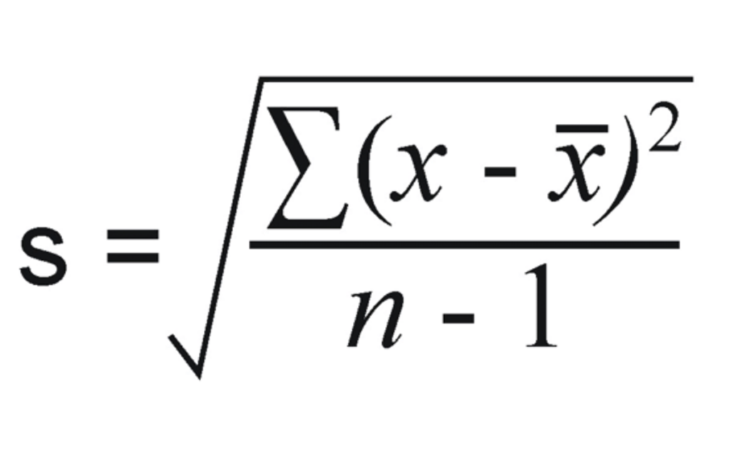
For example, with variance and standard deviation, observe the following problem: We are going to compare the two different 1-dimensional data sets. The first data points are [3, 6, 9], and the second data points are [1, 2, 3].
Before even computing, we are able to see that the second data point has a lower variance. They all congregate toward the mean. All values are within 1 of the mean in data set 2. There is higher variance in the first data set since all values are within 3 of the mean.
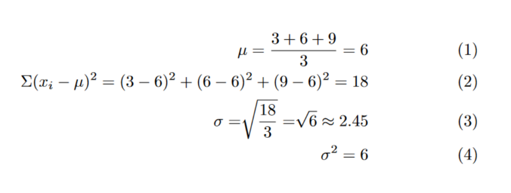
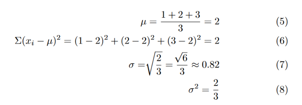
Standard deviation and variance allow you to better understand the center of your data. The variance will tell you how well your average actually represents the data. Refer to the following example:
Let’s say there is a rating system that goes from 0 to 5 stars. Blue dots represent a review of that number of stars.
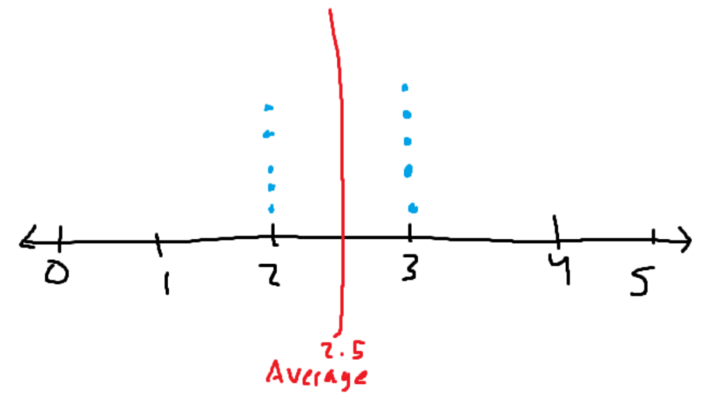
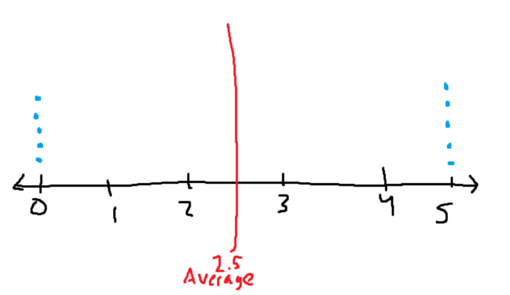
Both images have the same average of two and a half stars. In the first image, the mean does a good job of describing the entire data set. All of the data is close to the average value of 2.5. In the second dataset, the average poorly describes the entire data set. It says that the average is 2.5 stars, despite the fact that the only ratings given were either 0 or 5 stars. The average is in the middle of the data, where no data points are even remotely close to it.
The first data set has low variance, while the second data set has extremely high variance. The high variance causes the data to be inaccurately described using the average or other methods of getting the center of the data.
The normal distribution (or Gaussian Distribution) is one of the most important functions in all of statistics. The normal distribution is a continuous probability distribution. The normal distribution models the bell-shaped curve.
The formula is above, but it’s not of utmost importance to memorize it. As mentioned, the normal distribution models a bell curve.
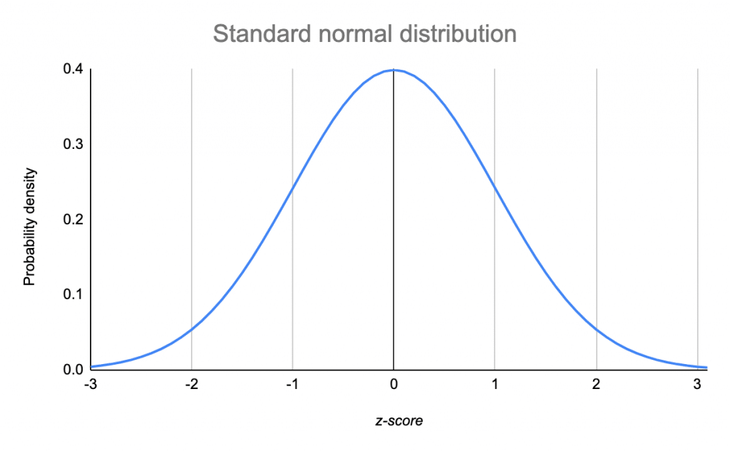
The normal distribution is a probability density function (PDF). It models the probability of a certain value appearing. By the definition of a PDF, the entire area under the graph will always be 1 (more formally, the improper integral from -inf to +inf is 1). The key property of PDFs is that the area under the graph describes the probability of an event occurring.
For example, getting the area under the curve along the interval [2, 5] will give the probability that a datapoint will land between 2 and 5 for that given normal distribution. As some may know, you can get the area by using integrals. Here is the equation for calculating the exact probability:
Doing the integral will always give you the exact answer. But approximation can be way faster than typing the full integral into a calculator.
Standard Deviation and Normal Curves
As mentioned earlier, a normal curve can be defined by its mean value and its standard deviation.
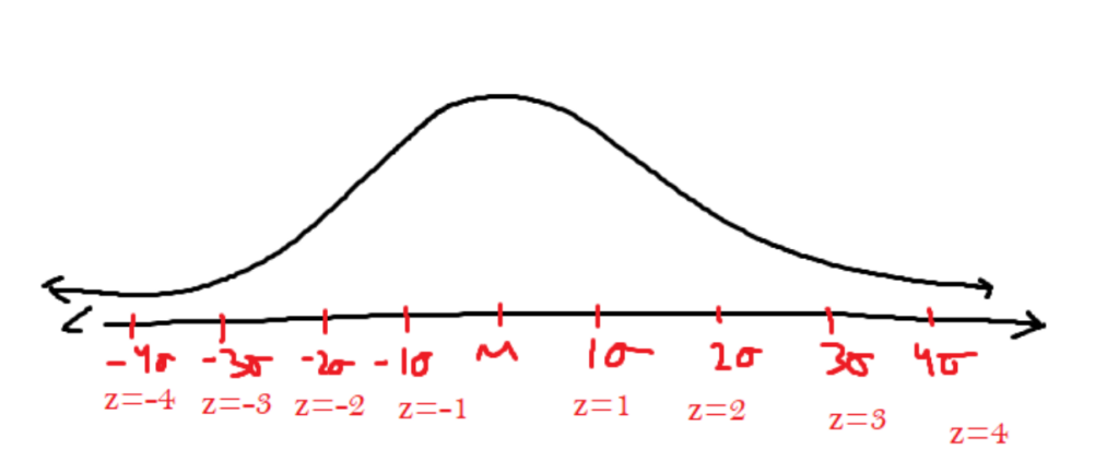
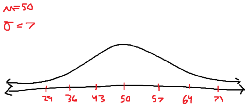
The image describes the number of standard deviations a certain part of the function lies away from the mean of the function. The normal curve is symmetrical. So, there exist two different points where it is 1 standard deviation away from the average. In order to differentiate, we use the z-score, which is the signed standard deviation. If you’re left of the mean, the z score will be negative, and if you’re on the right of the mean, the z score will be positive.
There are z scores that aren’t integers. A z score of 1.65 says about the x value, which is 1.65 standard deviations to the right of the mean. The area under the curve is the probability of the data appearing within that range. There are shortcuts for determining values that land on integer standard deviations.
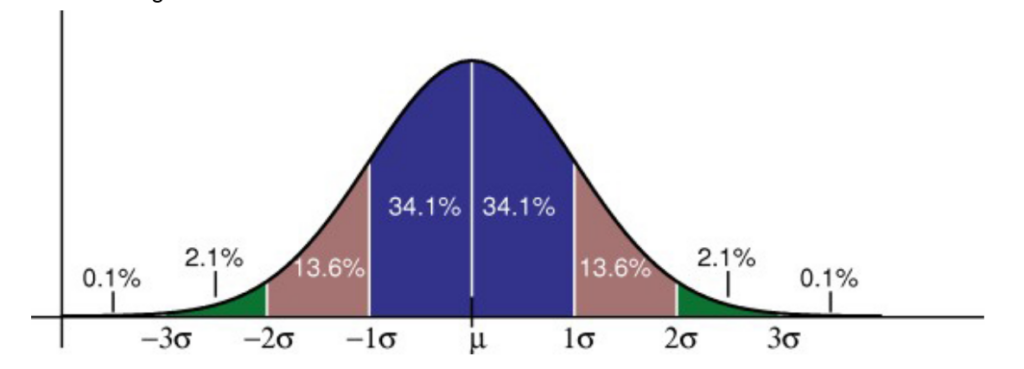
Some facts that can be obtained through the graph are:
- According to the drawing, the probability of data landing in between the mean and z = 1 is roughly 34.1%.
- There is approximately a 68.2% chance of the data landing within the first standard deviation.
- There is also approximately an 81.8% chance of data landing between z = -2 and z = 1 in a normal curve.
This is great for quickly identifying the probability of a data point landing within integer z-scores. To approximate, in problems where z scores aren’t integers, a normal distribution table will have to be used. The following are the normal distribution tables for positive z scores and negative z scores.
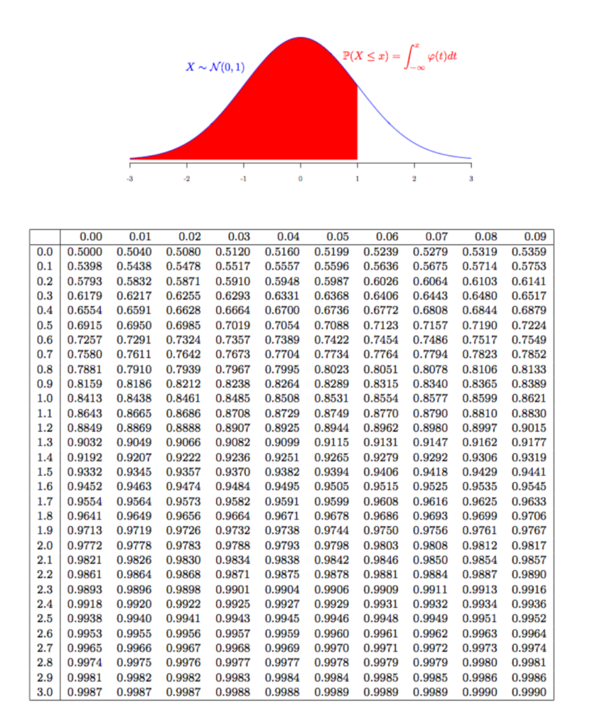
The table will allow you to get information on z scores up to the hundredth place. To use it, first find the closest z score to your value on the vertical axis. Once you find that value, go across the horizontal axis until you find the closest hundredths value.
The values in the normal distribution table will give you the area to the left of that z score. If you have a z score of 1.22, then the portion to your left has an area of 0.8888. With this information, you can determine that there is an 88.88% chance of a value landing on the left side of z = 1.22.
To determine the chance of the value being on the right side of a z score, it’s as simple as 1 (value in the table). Since the total curve has an area of 1, subtracting the left side area will leave you with the right side area.
For getting an interval in the middle of the curve. Get the areas to the left of each z score. Then, subtract the smaller area from the larger area to get the area in between.
Relationship between the z score, the x values,the average, and the standard deviation
The z score, x values, average, and standard deviations are all tied together in the following equation. This equation will come in handy for a lot of problems ( I do not contribute to either of these posts)
https://www.statisticshowto.com/probability-and-statistics/statistics-definitions/empirical-rule-2/
Binomial Distribution
Binomial Distribution
Binomial distribution talks about the probability of a certain outcome when there are only two events. A success event and a failure event If you toss a coin with the intent of getting heads, then getting heads is a success event, and getting tails is a failure event. If you’re rolling a die for 5’s, then getting a 5 is a success event, and getting any other number is all grouped together into one failure event.
The following formula is the formula that will be used to solve binomial distribution probability problems.

The first portion of the formula, which says n chooses x, is a reference to the combinations formula. Where you will be plugging the values n and x into.
Explanation of the formula:
(p^k) * (q^(n-k)) says find the probability of having k successes and the rest of the sample test cases be failures. Since there are usually multiple different ways of obtaining k successes and n-k failures (by changing the order of when you get your k successes), you need to find all possible combinations. Right now, you are only accounting for one way to get k successes from n samples. You would have to calculate how many samples of length k there are in n (combinations formula). Multiplying that value by the probability will give you the probability of getting a combination with k successes.
The following example is given at the following prompt:
If you roll a die 12 times, what is the probability that you will roll exactly 5 sixes?
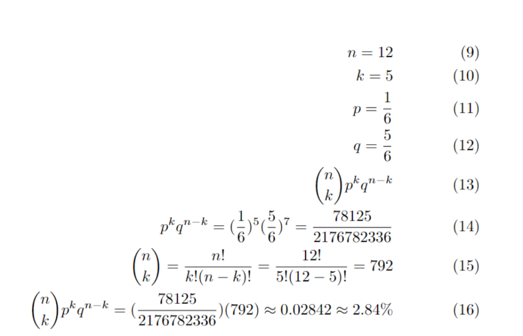
This can be expanded to getting the probability of rolling 6 at most 5 times. You just need to use the binomial distribution formula and get the probability of rolling a 6 0, 1, 2, 3, 4, and 5 times.
P(x<=5) =P(0) + P(1) + P(2) + P(3) + P(4) + P(5)
This also works for getting rolling six more than five times.
P(x>5) = P(6) + P(7) … + P(12)You could even expand this even more to get the probability of rolling 6 more than 3 times but less than 7 times.
P(3<x<7) = P(4) + P(5) + P(6)
Here are some other important formulas for dealing with the properties of binomial distributions. How to calculate mean, variance, and standard deviation (formulas are in the same order as this)
Geometric Distrubtions
The geometric distribution is another probability density function. The geometric distribution, similar to the binomial distribution, has two outcomes for each trial: success or failure. Geometric distribution describes the probability of a success event happening after a certain number of failures.
Geometric distribution is simple, and its formula comes easily after an example:
Calculate the probability on a 6-sided die of rolling your first 4 on your 5th roll.
We know that the probability of not getting a 4 is ⅚, and the probability of getting a 4 is ⅙. So most people will logically do the following:
This represents multiplying the probability of failing four times by multiplying the probability of getting one success. This is correct, and the formula just generalizes it. The formula is the following:
Geometric distribution models exponential decay because the more failures, the more fractions you multiply together.
https://www.desmos.com/calculator/t1uhsihoiu
The equation gets even easier when given a problem like the following:
What is the probability of rolling one 4 within five rolls of a six-sided die?
When dealing with the next problem, the equation gets even simpler than before.
What is the probability of getting your first 4 after your first 5 rolls of a six-sided die?
This is the equivalent of just failing five times, so the equation is the following:
Here are some other important formulas for dealing with the properties of geometric distributions. How to calculate mean, variance, and standard deviation (formulas are in the same order as this)
Poisson Distribution
Poisson distribution represents the probability of a certain event occurring based on how often that event has occurred in the past. An example problem might be the following:
Every hour, on average, 11 boats pass the lighthouse. Calculate the probability of seeing 25 boats pass in 2 hours.
The formula for calculating the poisson distribution is the following:

The formula is pretty simple but there is one thing that needs to be taken care of prior to plugging in the values. Notice in the above problem 11 boats pass the light every ONE hour. Calculate the probability of seeing 25 boats pass in TWO hours. Instead of making the mu equal to 11 you need to make mu equal 22. The time intervals must be the same for the equation to work. This means you might need proportion equations to how much to change your mean in more complex problems.
Below is a website which talks more about posson distributions (I do not own this website)
https://rachelchen0104.medium.com/statistics-101-binomial-and-poisson-distribution-af4f3cf3e774
Uniform Distribution
A uniform distribution is a probability distribution where every single outcome has an equal chance of occurring. There is a uniform probability. One example of this might be the chance of rolling each number on a fair six-sided die. Each side has a ⅙ chance of occurring.
Since every outcome has an equal probability of occurring, the graph of a uniform distribution is usually some sort of rectangle.
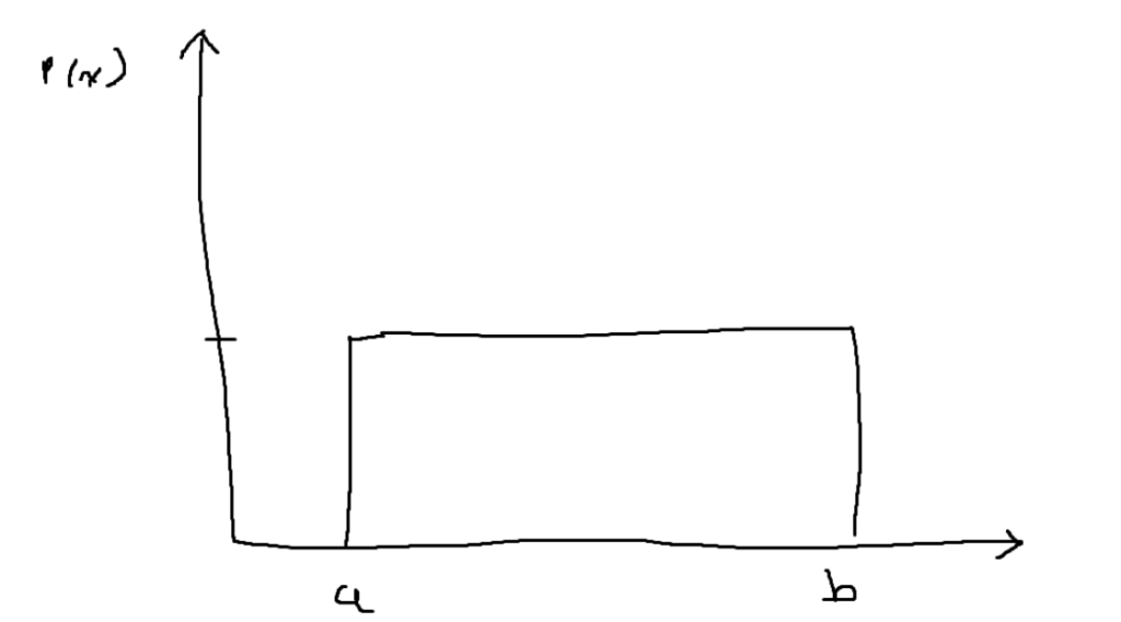
A uniform distribution is a probability density function. This means that it has a total area of 1, and the area under the curve represents the probability. Conveniently, getting the area of the rectangle is as simple as using A = bh.
In most scenarios, you are given the range of the outcomes (spanning from a to b in the image). However, it might be up to you to figure out the height of the uniform distribution graph. The horizontal length of the rectangle is rewritten as b-a. We also know that the whole rectangle must have an area of 1. This leaves you with the equation 1 = (b-a)(h), and with a little bit of algebraic manipulation, you will end up with h = 1/(b-a). Every value in the range from a to b will have a probability of occurring equal to the height of the graph.
The following graph describes the probability of a value landing between 20 and 30. Where a = 10 and b = 40.
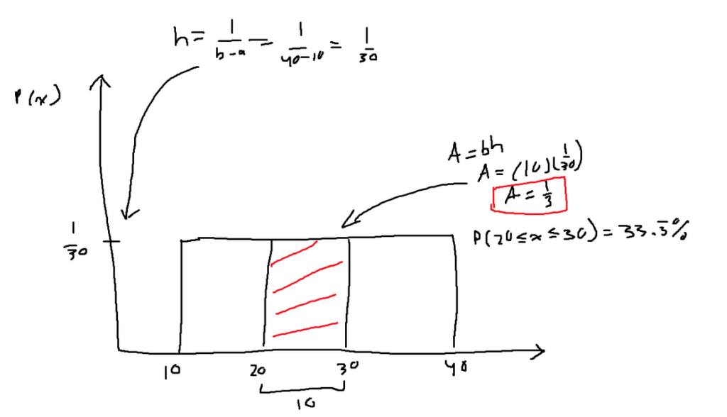
This really is just for finding the probability within a range for data that is uniformly distributed.
It shouldn’t be that surprising that the median and the mean have the same value because of the equal distribution. The mean and median are both located halfway between a and b.
Exponential Distribution
Exponential distribution:
Exponential distributions are another type of probability distribution. Exponential distributions usually deal with time. An example might be dealing with the life expectancy of certain products, which usually follows an exponential distribution. A question might determine the probability that, after X years, some certain product is still working.
All exponential distributions can be represented by the following function: Lambda is called the rate parameter; it is the only part of the function that differentiates exponential distributions. Lambda will also always be the y-intercept of the graph.
An exponential distribution is an example of a probability density function. This means that the total area under the curve is exactly equal to 1, and the area under the curve of a certain region is equal to the probability of data being found there.
Since all of the exponential distributions are extremely similar, People have created the following general formula for finding the area under the curve of exponential distributions:
The first formula for getting the area to the left of a certain value
The second formula for getting the area to the right of a certain value
These formulas aren’t that hard to obtain. By integrating the general formula of an exponential distribution, the two above formulas can be confirmed.
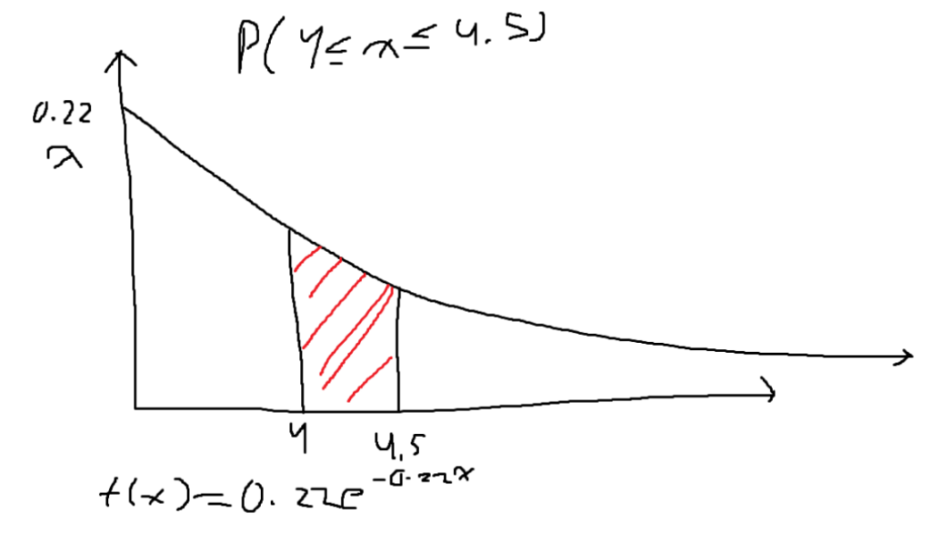
Below is the solution for finding the area of the shaded red area in the image above.
Some extra formulas:
The mean of an exponential distribution can be found using the following formula: The following formula can be derived from the general function by solving the integral found under the formula.
The variance can be found using a very similar formula to the prior one. It can be rediscovered by solving the integral under the variation formula.
Now that you have the variation formula, you can derive the formula for the standard deviation. The variance is just the standard deviation squared. Which means that the standard deviation of an exponential distribution is equal to the mean of an exponential distribution.
Confidence Interval and Margin Of Error
Confidence intervals are used when trying to reflect sample data onto a larger population. When you take samples of a population, they will usually not perfectly represent the entire population. Let’s say a sample has a sample mean of 50. You cannot assume that the entire population has a population mean of 50. A confidence interval describes a range of values that sprout from your sample mean of 50. If you have a confidence level of 90% for your confidence range, Then, if you took more samples of the same size, there would be a 90% chance that their sample means would land inside that confidence range.
The concept is better explained with an example problem:
Let’s assume we need to find the confidence interval that has a confidence level of 90% using the following information:
The confidence interval is defined as follows (each part will be explained later):
We already know the sample mean, so let’s just look at the margin of error portion, which is the second term. For the margin of error equation, we know all but z-alpha. Z alpha is really just the z score.
Using the z score table, we can turn an area into a z score. The area to the left of the currently unknown z score is the following:
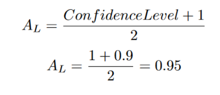
This means that the area to the left of our z score is 0.95. By searching for that area in the z score table, we can get back the z score. (I do not own the following website)
https://www.mathcelebrity.com/zcritical.php?a=0.95&pl=Calculate+Critical+Z+Value
Our z score for this problem is 1.64. By plugging in the values, we will get our margin of error for this problem.
We now have all the parts that are needed to construct a confidence interval of 90%.
We have the confidence interval, but what does it mean? If we continued to take more samples of size 20 and measured their averages, then 90% of them would fall into our confidence interval.
Our confidence interval wasn’t very big. This is partially due to the fact that our confidence level was 90%. Had our confidence level been a value like 95% or 99% (the z score would have been bigger), our confidence interval would have spanned farther.
Chebyshev’s Theorem
Chebyshev’s Theorem is able to predict the minimum area that is encapsulated by any type of distribution for a specific standard deviation. It is able to predict the absolute bare minimum probability that a value will land in between k standard deviations from the mean. Chebyshev’s formula is as follows:
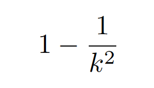
One caveat of Chebyshev’s formula is that your k has to be greater than 1. If you try plugging in a number smaller than 1 for k, the formula doesn’t predict values correctly.
As mentioned before, Chebyshev’s formula works on all types of graphs. If the initial definition was confusing, refer to the following example:
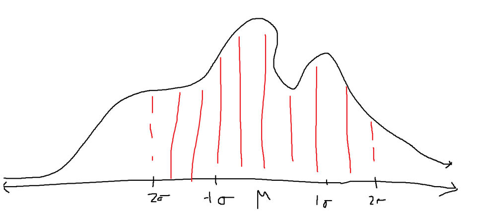
Assume the above function is a probability density function (the total area under the curve is 1, and the area under the curve of a certain range is the probability of landing inside that range). We don’t know the area of the red-shaded region, which is also the area between two standard deviations of the mean. The graph also doesn’t represent any of the common distributions, like a normal distribution, so we can’t use any of those formulas.
The only information we can extract is the minimum area of the red-shaded area. If we plug in k equal to 2 (representing the 2 standard deviations), we will get the following:
We get back that the minimum area of the shaded red region is 0.75. That means there is at least a 75% probability that a value lands within 2 standard deviations of the mean in this specific problem. The true probability might be 80%, 90%, etc., but we know that the true probability will always be above 75%.
Null and Alternative Hypothesis
There are two different types of hypotheses. The first is called the null hypothesis, and the second is called the alternative hypothesis.
The null hypothesis, denoted by (Ho), is the currently accepted answer for a metric of a population.
The alternative hypothesis, denoted by (Ha), is a new claim that challenges the null hypothesis.
The hypothesis can either be in the context of an average or some sort of proportion.
Example 1(Mean):
I believe that the average age in my town is 25 years old. However, my friend disagrees with me and starts surveying people.
The null hypothesis would be the belief that the average age in my town is 25 years old.
The alternative hypothesis would be the belief that the average age in my town was not 25 years old.
Example 2 (proportion):
I believe that at least 50% of people in my town have a driver’s license. However, my friend disagrees with me.
The null hypothesis would be the belief that at least 50% (P >= 0.5) of the people in my town have a driver’s license.
The alternative hypothesis would be the belief that no more than 50% (P < 0.5) of the people in my town have a driver’s license.
One and Two Tailed Tests
For testing an alternative hypothesis, there are two different types of tests (technically three) that are used to determine whether the alternative hypothesis should be adopted. The two tests are called one-tail tests and two-tail tests. Each is used in different scenarios.
Two-tailed tests should be used when the alternative hypothesis claims that the null hypothesis is not a specific value.
Example:
Ho: mean equals 10
Ha: The mean does not equal 10.
The null hypothesis makes a claim that the mean is equal to 10. While the alternative hypothesis makes a claim that the mean is not 10,
A two-tailed test will look something like the graph below. The variable alpha is (1, the confidence level). The confidence level is decided by the person developing the alternative hypothesis. Sprouting from the mean of the normal distribution, there is an area equal to 1 alpha in decimal form (1-0.05 = 0.95 if the confidence level is 95%).
There are two red-shaded areas. Each has an area of alpha / 2 (for 95%, that would be 0.25 each). While testing a hypothesis, a new testing z score will be found (this is talked about in the following section). If the new testing z score is found inside the red-shaded area, then the null hypothesis should be rejected and the alternative hypothesis should be adopted. If the new testing z score is found inside the white space, then the null hypothesis has failed to be rejected and should be kept.
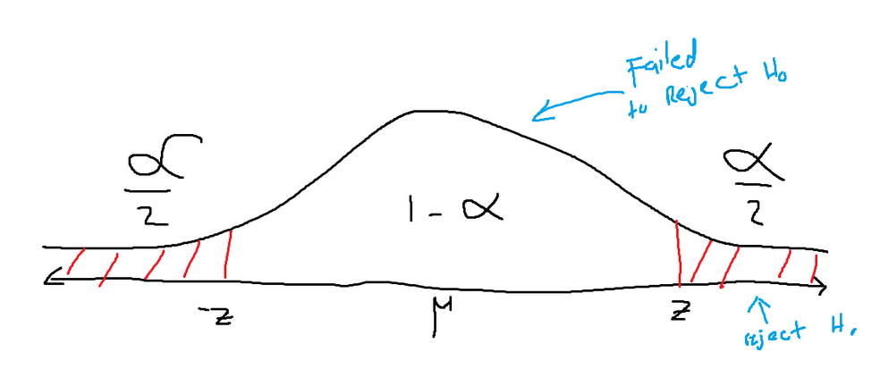
The rejection zone is decided by two symmetrical z scores. These two points are called the critical points.
One-tailed tests should be used when the null hypothesis claims that the current range is either too high or too low. Some examples might include:
Note: P means proportion (like 50%, 75%, etc.) and is represented by a value between 0 and 1.
Example 1:
Ho: P >= 0.5
Ha: P< 0.5
The null hypothesis makes a claim that the proportion is greater than or equal to 50%. While the alternative hypothesis makes a claim that the proportion is actually less than 50%,
Example 2:
Ho: P <= 0.3
Ha: P > 0.3
The null hypothesis makes a claim that the proportion is less than or equal to 30%. While the alternative hypothesis makes a claim that the proportion is actually greater than 305,
There are two different types of one-tailed tests. Example 1 is an example of a left-tailed test, and Example 2 is an example of a right-tailed test.
Below is an example of a right-tailed test. The meanings of all the values are the same as what was mentioned for the two tail tests. However, since there is only one tail, the area of the one tail is alpha.
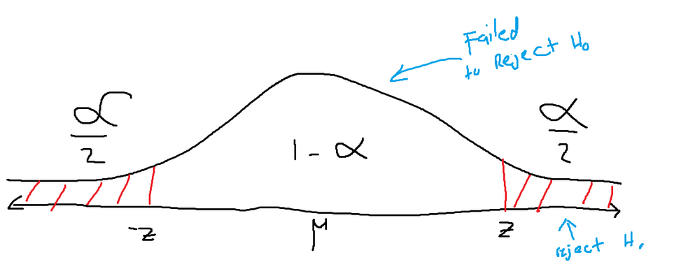
To figure out whether the alternative hypothesis is better than the null hypothesis, an experimental z value will be found using the new data that was collected. If that newly calculated z score lands inside the red-shaded area, then the null hypothesis should be rejected. If not, then the null hypothesis should be kept.
When trying to disprove a null hypothesis, sample data will be collected and used to determine whether the current hypothesis should be changed.
For scenarios dealing with means:
If n<30 and the population standard deviation is unknown, then the student t-distribution should be used to approximate. (t score)
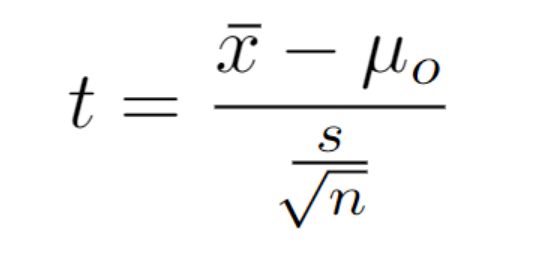
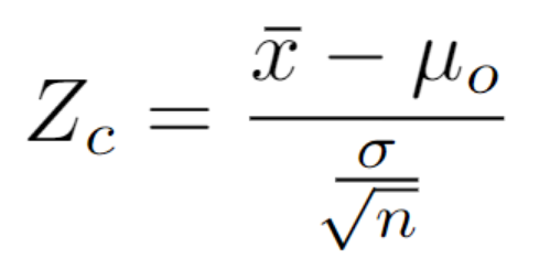
If n<30 but the population standard deviation is known, then the normal distribution can be used to approximate. (z score)
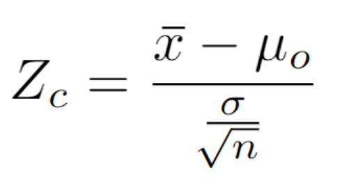
If n > 30 (the sample size is sufficiently large) and the standard deviation is unknown, the normal distribution can be used to approximate the z score.
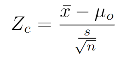
If n > 30 and the standard deviation is known the normal distribution can be used to approximate (z score)
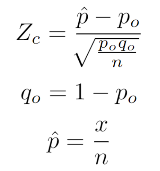
For scenarios dealing with proportions:
Example 1 (using Z-Score):
I claim that the average age of people in my town is 33 years old. However, my friends disagree and believe that the average number of people in my town is not 33. He does some research to prove his claim. He sampled a total of 50 people and found his sample mean to be 31. The standard deviation of the data he collected was 2.1. Use a 95% confidence level.
Null Hypothesis: mean = 33
Alternative Hypothesis: mean = 33
First, we need to determine what type of test we have. In our scenario, our alternative hypothesis is an inequality, so it is most likely a two-tailed test.
Since we have a sufficiently large n (n > 30) but don’t know the population standard deviation, we will use the z-distribution formula with the sampling standard deviation (3rd formula).
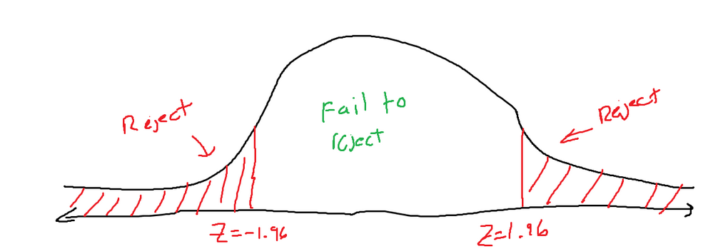
We know that the significance is 0.05 (1 + 0.95). Since we have a two-tailed test, we know that alpha will be split evenly between each tail. Which means we need to find the z-score, which correlates to an area to the left of 0.975 (1 – (0.05 / 2)). That z-score turns out to be 1.96. So, our graph currently looks like the following:
Now we need to plug our values into the equation. If you read through the word problem, we can figure out our givens.
Sample Average (x bar) = 31
Population Average (mu) = 33
Sample standard deviation (s) = 2.1
N = 50
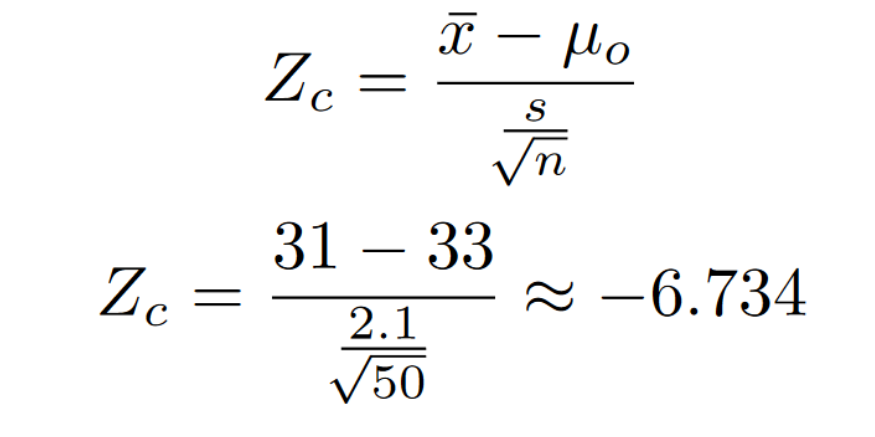
If you locate the z-score on the graph, You can see that the z score lands inside the rejection zone (Z < -1.96 or Z > 1.96). This means that the null hypothesis should be rejected. My friend has sufficient evidence to prove his point that the mean is, in fact, not 33.
Example 2 (using a T-score):
I make the claim that the average lifespan of a frog is at least 5 years. My friend thinks frogs don’t live as long. He chooses to collect data to prove his point. He tested 20 frogs, and they had an average lifespan of 4.8. The standard deviation of his data was 1.9. With a confidence level of 95%.
Null Hypothesis: mean >= 5
Alternative Hypothesis: mean < 5
We again need to determine what type of test we have. We have an inequality that cuts the possible tests to two one-tailed tests. We can see that our alternative hypothesis predicts a value lower than the current mean. So, if we were going to find a better value, it would be on the left. We should use a left-tailed test.
Since we don’t have a very large n (n <= 30) and we don’t know the population standard deviation, we will have to use the t-distribution to find our answers. Don’t mix up the t-distribution with the normal distribution. T-distribution is used for dealing with samples and smaller-sized information.
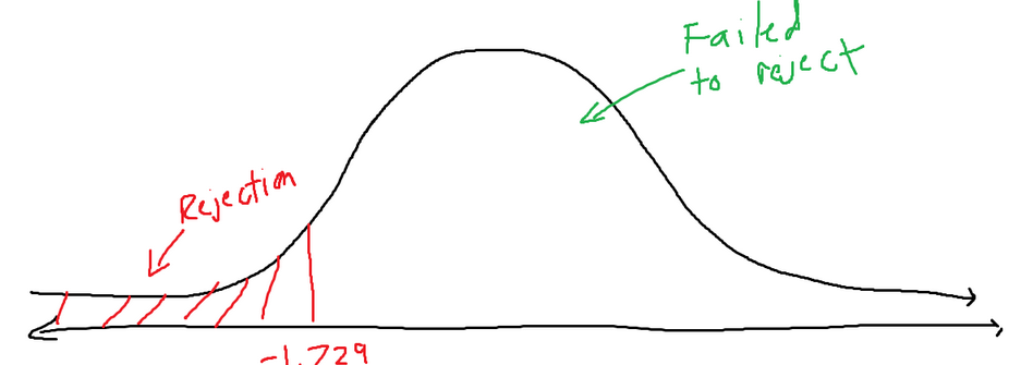
We know that we have a significance value (the variable alpha) of 0.05 (1-00.95). We have a left-tailed test, so the left tail has an area equal to alpha. We need to find the critical value that separates the rejection zone from the failed-to-reject zone.
We have 19 degrees of freedom (df = n-1) and a significance of 0.05. We can figure out that our t-score value is -1.729. If you search for these values, you will find 1.729. 1.729 represents the t-score according to a 0.05 significance level from the right. We want it to be to the left, so simply make it negative because the t-score distribution is symmetrical.
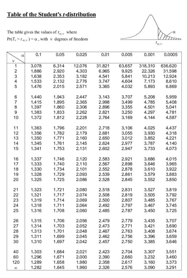
Our current t-distribution graph looks like the following:
Now we need to plug our values into the equation. If you read through the word problem, we can figure out our givens.
N = 20
Population average (mu) = 5
Sample average (x bar) = 4.8
Sample standard deviation (s) = 1.9
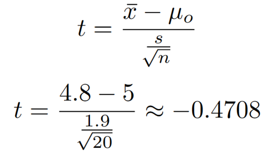
We realize that our t-score landed outside of the rejection zone. This means that the alternative hypothesis failed to reject the null hypothesis. In other words, the belief that the average age of a frog is over 5 should be maintained.
Example 3 (when there is a proportion)
I believe that 68% of people in my town are over the age of 20. However, my friend thinks differently and chooses to collect some data. He tested a total of 500 people. He found that in the sample, 360 of the total 500 people said they were over the age of 20. Use a 95% confidence level.
Null hypothesis: 68% of people in my town are above the age of 20 (age = 68).
Alternative hypothesis: The proportion of people in my town that are older than 20 is not 68%. (age = 68)
The alternative hypothesis states that the age proportion is not a specific value. This means we have a two-tailed test.
When dealing with proportion, we will use a normal distribution and z-scores to figure out whether the null hypothesis should be rejected. The problem states that we should use a 95% confidence level. Using the z-score table, we can figure out where our critical values are (the points that separate the rejection zone).
An important thing to note is that this is a two-tailed test. So each tail has an area equal to the significance value (1- 0.95) divided by 2. Refer to the image for more information.
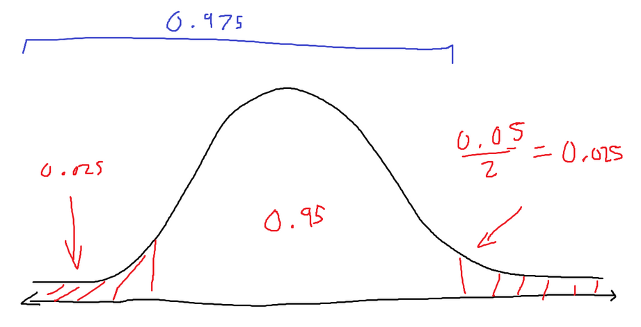
We need to search for the z-score, which has an area equal to 0.95 (confidence level) + 0.025 (alpha / 2), or 0.975. We find in the z-score table that the value that best satisfies that area is the z-score of 1.96. There is a critical point at z = 1.96, but there is also a critical point at z = 1.96. Since we are using a two-tailed test,
In this problem, we are using proportions, so we will have to use the only proportions formula. From the problem statement, we can extract the following:
P Initial = 0.68 (same thing as 70%)
Q Initial = 0.32 (1 – 0.68)
P is usually associated with the probability of something being true (in this case, being over 20). Q is the chance of the probability of something being false, so it can be found by p if there only exist two outcomes.
We need to calculate the percentage of being over 20 in the sample (the P-hat variable).

Now that we know the percentage of being over 20 in the sample, we can plug all of our values into the formula to figure out what our z-score is.
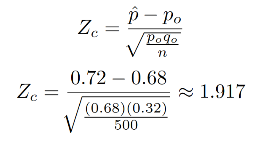
Our Z scores don’t land inside the rejection zone (it is a super close thought). This means that the alternative hypothesis failed to reject the null hypothesis. In other words, the belief that 68% of my town is above the age of 20 should be kept.
Cohen’s D
The Cohen’s D test is used to determine the size of an effect. The Cohen’s D test works with the difference in the means of the distributions. A use of Cohen’s D might include figuring out which marketing strategy has a bigger impact on total sales. Or determining which teaching method affects the students the most.
The d-value will always be expressed in terms of standard deviations. The bigger the d-value, the bigger the difference there is between their means. In most scenarios, around 0.2 is considered a small impact, around 0.5 is considered a medium impact, and around 0.8 is considered a large impact. Below is the formula for finding the d-value.
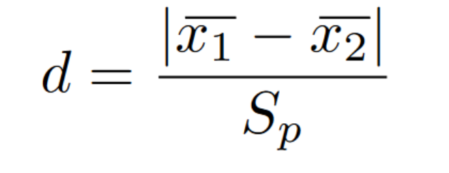
The variable in the denominator represents the pooled standard deviation. Since you are dealing with multiple distributions, there are also multiple standard deviations. Below is the formula for combining the two distributions to get their combined (or pooled) standard deviation.

Refer to the following example, where we solve for the d-value using the given values in the image:
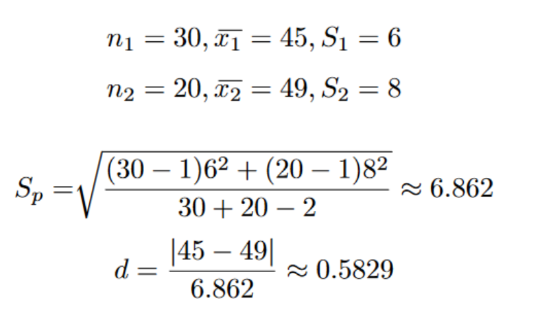
In the above example, when the two distributions are compared, they have a medium-level effect on each other.
Cohen’s D is highly susceptible to guessing a value above the true value. Which is why people tend to use Cohen’s D when the sample sizes are above 50. Some people also tried subtracting some from the d-value. There are also multiple other methods to calculate the impact. But refer to the following article: https://www.statisticshowto.com/cohens-d/.
When interpreting a d-value, you need to look at the bigger context. The d-value is just a number at the end of the day. When something has a low d-value, it does not necessarily mean it’s unimportant. If a new method of cancer treatment has an effect on patients with a magnitude of d = 0.2, it’s important in that context. Finding that a school’s new program has an impact of d = 0.2 isn’t as important as finding that it is impacted by a lot of other factors other than just the program.
Chi-Squared Test
Chi-Squared Test
The Chi-squared test is used to determine the goodness of fit. It finds a way to compare the observed and expected values of a certain distribution. Some examples might include determining whether a certain distribution is good enough to be approximated by a uniform distribution. The Chi-squared test is also used to determine whether a variable is independent of the values it produces.
The chi-square test is a hypothesis test on the chi-square distribution. The chi-square distribution looks close to a normal distribution, but it is slightly skewed to the left.
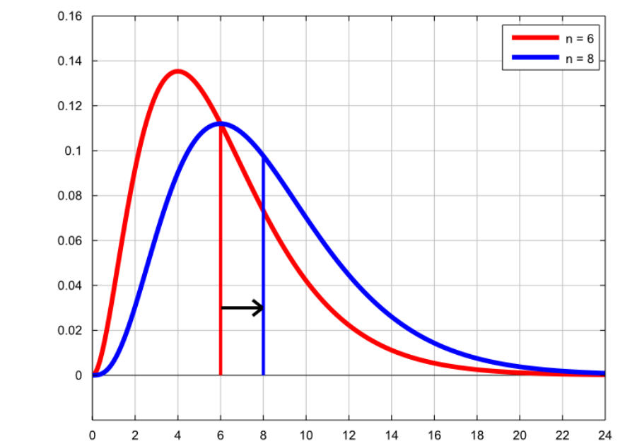
The chi-squared test works just like most other hypothesis tests. You need to determine a null hypothesis and an alternative hypothesis. Then, a critical value will be found, splitting the chi-squared distribution into a rejection zone and a fail-to-reject zone.
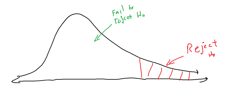
To find this critical value, the chi-square distribution table can be consulted. Below is an image of the table (Image Source):
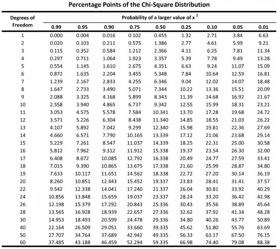
On the left-hand side, there is a degree of freedom. The degree of freedom is (total categories minus 1). For example, if you have weekdays (Monday, Tuesday, Wednesday, Thursday, and Friday), you have five total categories. So, the degree of freedom is four (5–1).
The top represents the area to the right of a critical point. This value will be the same as your significance (the variable alpha in most problems). If you’re not given significance, remember it can be calculated by your confidence level from 1.
Simply find the point where your degree of freedom and area to the right agree, and that is your critical value. If you have 22 degrees of freedom and a significance of 5%, your critical value is 33.92.
In order to calculate the chi squared, we will need an observed value and an expected value (this will be better explained in the first example). The formula for the chi-square of a distribution is the following:

Each observed value will have some sort of expected value tied to it, and you will use this pair for the calculations.
Based on the position in the graph of the newly calculated chi-squared value, we will decide whether to replace the null hypothesis. If the newly calculated point lands inside the rejection zone (defined by the critical value, which is talked about above), then the null hypothesis should be swapped with the alternative hypothesis. If the new value doesn’t land in the rejection zone, then the current null hypothesis should be kept.
Example 1:
Over the span of an entire year, a company earned a total of $1000. They split their year into four quarters. In the below table, there is the amount of money earned by the company in each quarter. Determine whether this information can be approximated to a uniform distribution with a 95% confidence level.
Quarter One: $287
Quarter Two:$223
Quarter Three: $265
Quarter Four: $225
One of the possible null hypotheses is the statement that the data represents a uniform distribution. In that case, the alternative hypothesis would be the statement that the data doesn’t represent a uniform distribution.
The problem states that we have a 95% confidence level. This means we have 0.05 significance. There are also four quarters, which means the degree of freedom is 3. If we look this value up in the chi-squared distribution table, we find the critical value to be 7.81.
Now for actually calculating the chi-squared value. We were given the observed values, but what are the expected values? If the distribution is assumed to be a uniform distribution, then each quarter should have an equal value. Which means the expected value for each should be $250.

We get that the chi-squared value is roughly equal to 11.792. If we compare this value to our critical value, We notice that our value lies inside the rejection zone. This means that our distribution should not be approximated by a uniform distribution.
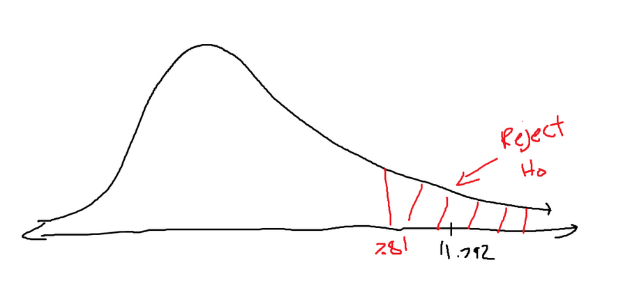
This might mean that sales have something to do with seasons or certain events that happen in each quarter.
Chi-Squared Distribution for Standard Deviation and Variance:
I’m too lazy to teach this, and the sources do a better job anyway.
In the following video, he uses the chi-squared test to determine whether a certain standard deviation value is a good fit for representing a specific distribution.
https://www.youtube.com/watch?v=O6a76Dnn104&list=PL0o_zxa4K1BVsziIRdfv4Hl4UIqDZhXWV&index=67
Chi-Squared distribution of testing independence:
I’m too lazy to teach this, and the sources do a better job anyway.
In the following video, he uses information that is formatted in a table. In the example I gave, we weren’t comparing anything. We were just determining whether this distribution was close enough to uniform. In the below video, he describes a scenario where he is determining whether two variables act independently of each other. Refer to my independent vs. dependent section.
https://www.youtube.com/watch?v=y5nxiL6civU&list=PL0o_zxa4K1BVsziIRdfv4Hl4UIqDZhXWV&index=68