Bezier curves are an extremely common concept in computer graphics. Bezier curves find a way to visualize curves that are way too complicated to represent with mathematics.
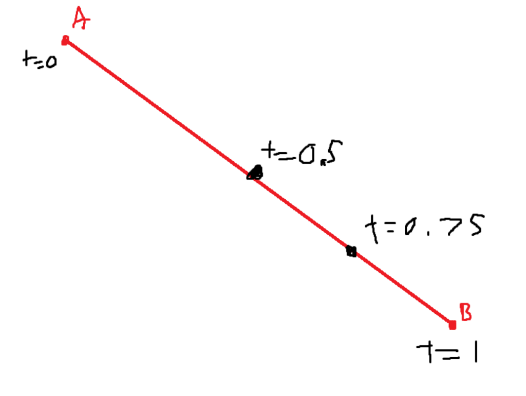
Bezier curves use the concept of linear interpolation. Let’s say we have points A, B, and the line segment that connects both of them. We can define another point on the line segment with a t-value. A number from 0 to 1 represents a ratio of its distance to either of the points.
If t = 0, then the new point is at the same spot as point A.
If t = 1, then the new point is at the same spot as point B.
If t = 0.5, then the new point lies midway between point A and point B.
If t = 0.75, then the new point lies 75% of the entire distance of the line away from point A.
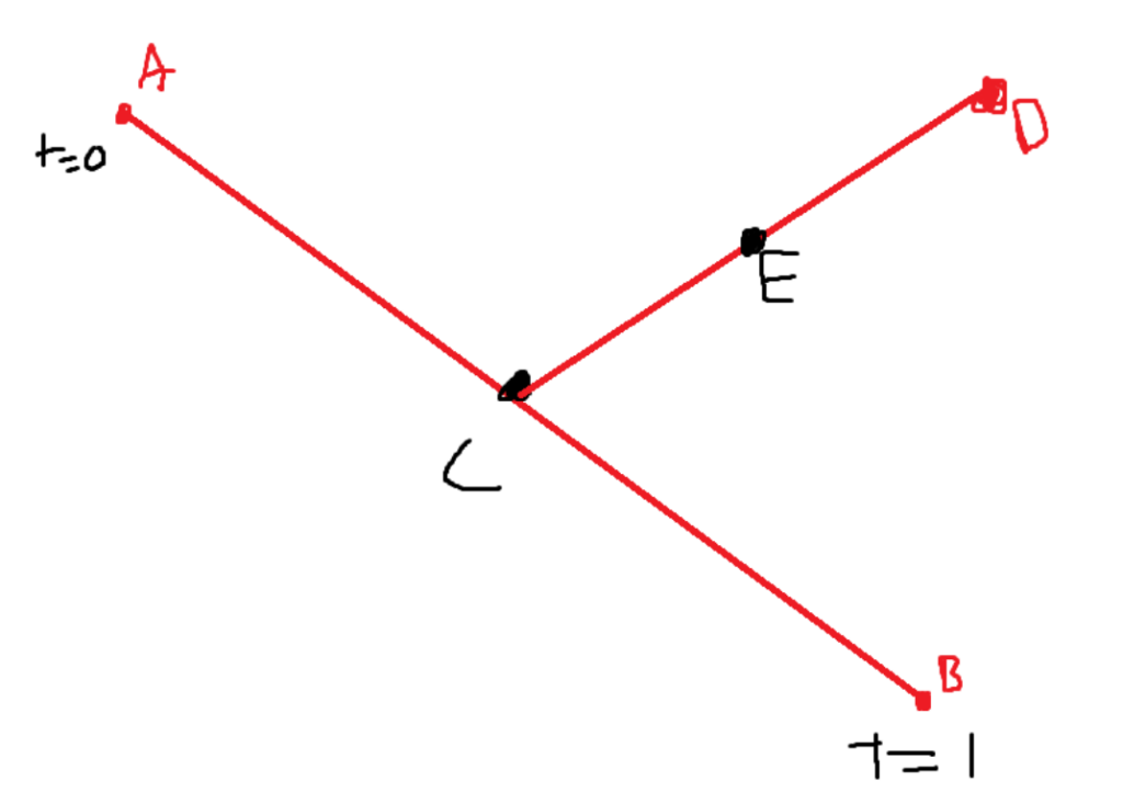
You can visualize this new point sliding around the line as the t value increases or decreases. Bezier curves rely on the idea of putting multiple t values together.
In the following curve, we have one point C sliding up and down on the AB line segment. Then, we have the line segment defined by that point C (which is still moving) and a fixed point D. On that line segment, we have point E, which is sliding along that moving line segment.
Enter the quadratic bezier curves. Which look like the following:
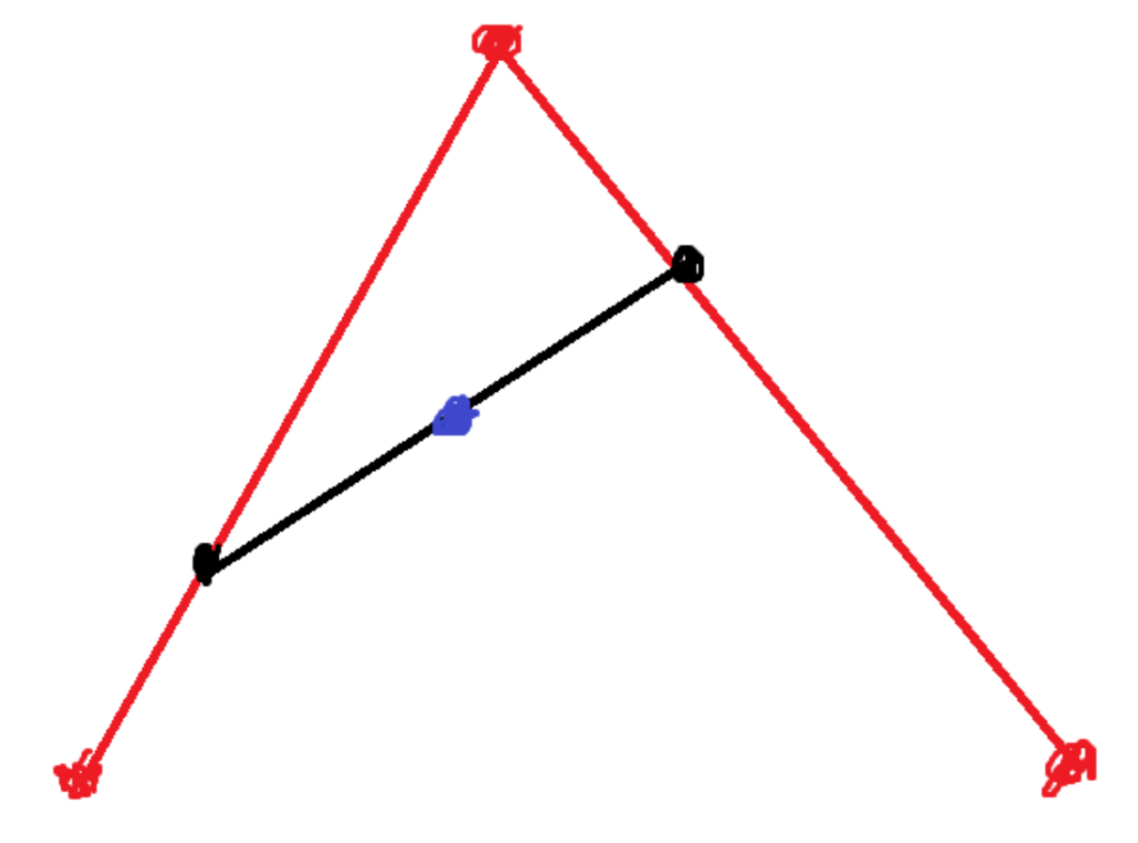
The red points are all fixed. The black points are sliding around the line segments between fixed points. The black points create another line segment with another point moving around on it (the blue point). The blue point is the point that draws the curves. The blue point’s positioning and therefore how the curve is drawn depend on multiple different factors.
It depends on where the black points are on their respective lines and where the blue point is on its line. Then, how the black points move depends on where the red points create the line at which they move. There is a lot of customizability even with a simple quadratic bezier curve.
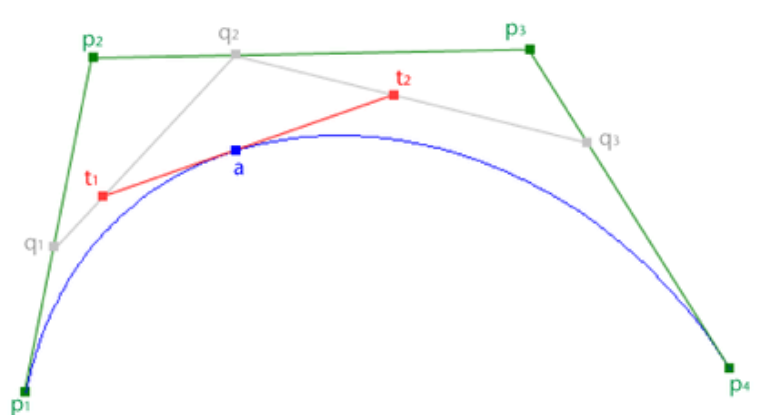
The most widely used bezier curve is the cubic curve, which looks like the following:
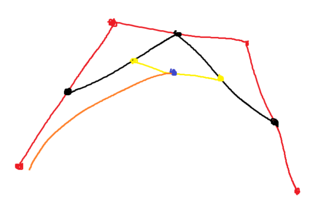
All points except the red points are moving around when drawing the curve. The red points can be moved around to alter the shape of the curve. Again, the blue dot is the point that draws the line, and the orange line is my best guess at what curve it might be drawing.
Mathematical interpretation:
The t-value defines the position of a point and represents some ratio on a line. We can write this behavior as an equation. Having it in a mathematical formula allows for even more functionality with bezier curves. Each moving point in a bezier curve will have an equation attached to it. Below is the general formula:

Refer to the following example:
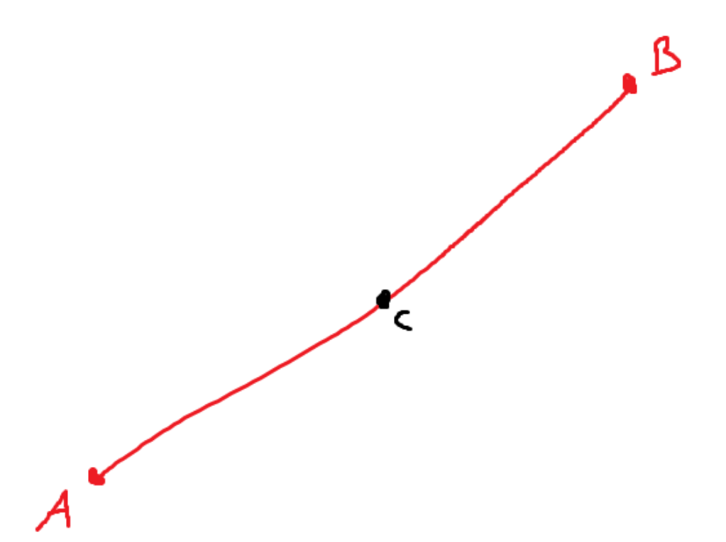
The location of C, given the t-value, will be determined by the following equation:

If we expand this definition to the cubic bezier, we can get the following:
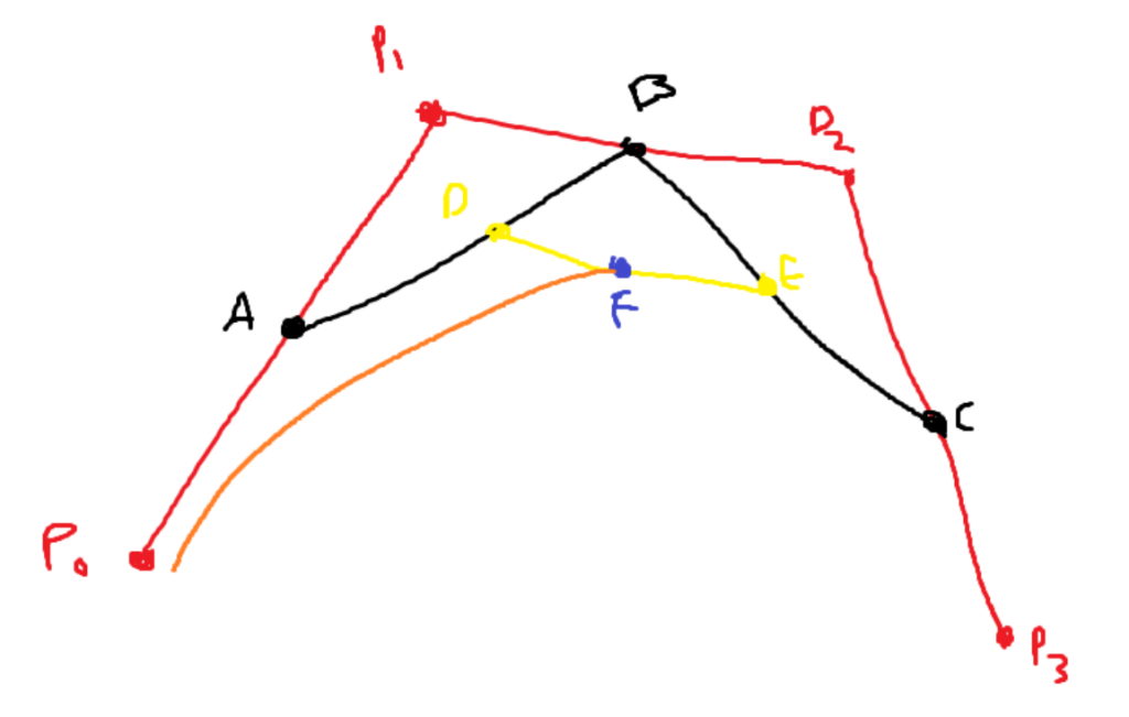
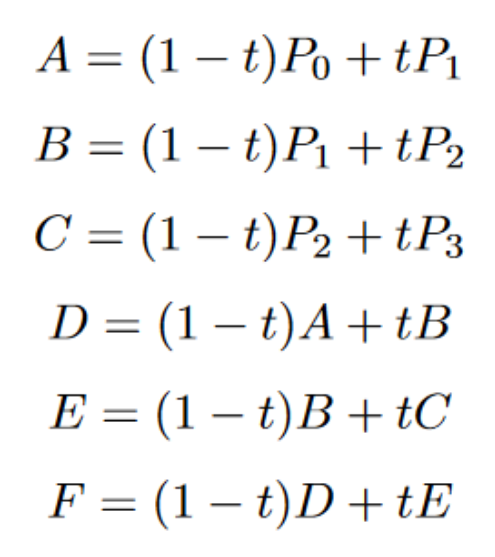
All fixed points (points 0–3) are vectors. If you take their vectors and put them tip to tail, you will get Point F. The point that draws the curve is a collection of all the vectors associated with each point. In the system of equations above, you are able to put a vector and a scalar multiplication into one term. Refer to the following, where the fixed points are “solved for”.

If you have the t-value, simply plug it in. Then, multiply them with their respective vectors.
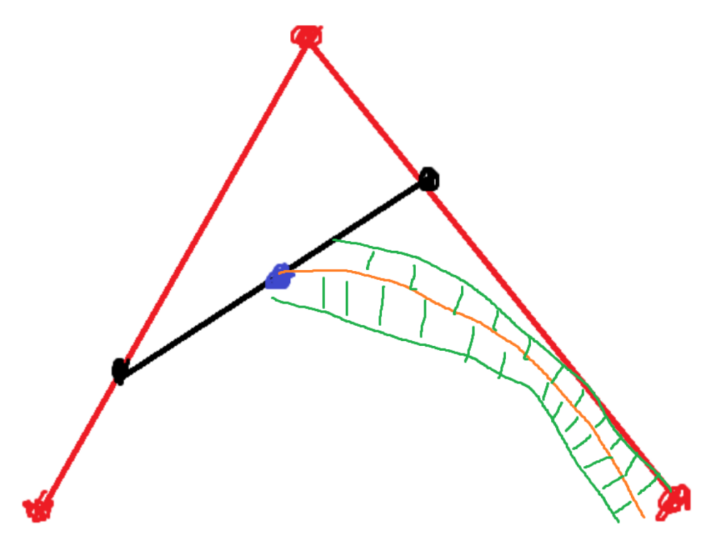
Having our curve defined by a summation of vectors allows us to add geometry to our bezier curve. Let’s say you are making a game and want to add physical geometry to your curve. Perhaps something like the following, where the green section represents a path.
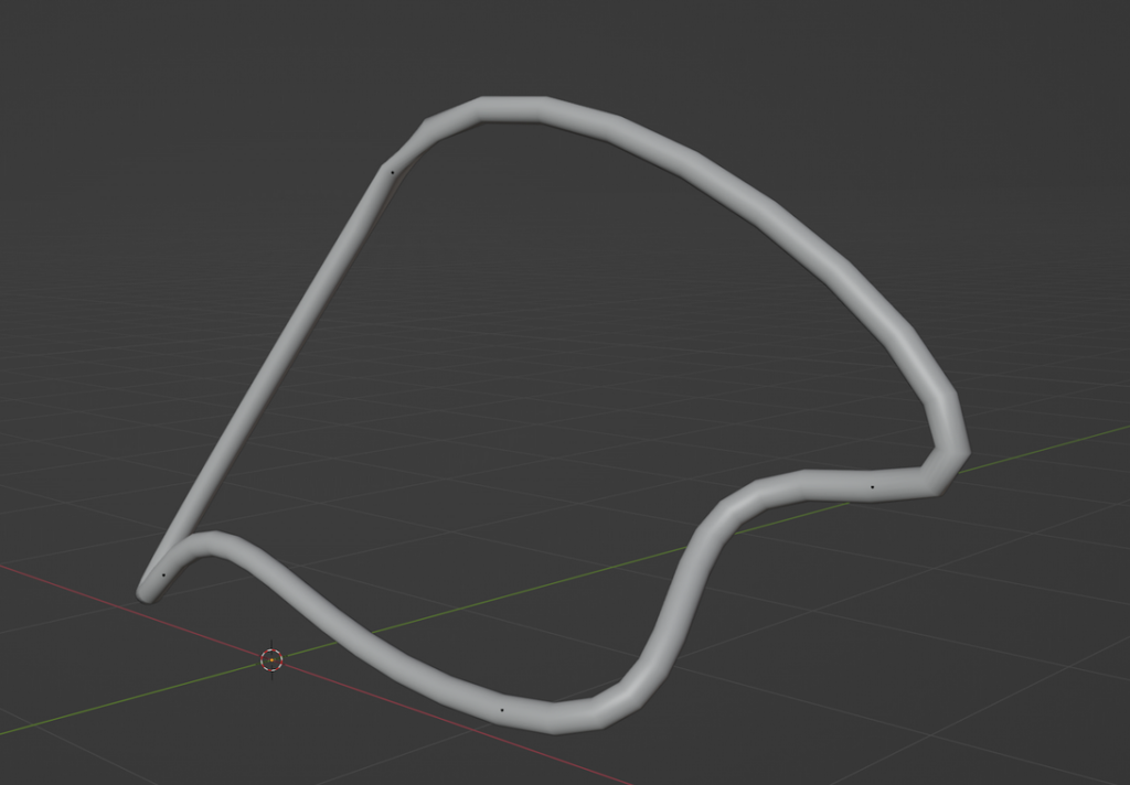
Or if that’s hard to visualize, below is a 3D model of a Bezier curve that has a path. The bezier curve traces a physical object out.
In most cases, it isn’t good enough to say that the path should surround the bezier curve. We need a mathematical definition for this. Most of the time, you want your path to be normal (perpendicular to the current) to the curve. In the following image, there are three vectors given (B is binormal, T is tangent, and N is a normal vector).
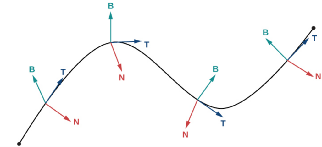
The normal vector will always point at a 90-degree angle away from the curve, and generally, that’s what we want for creating geometry. The tangent vector will always point in the direction of the curve. Finally, the binormal vector is defined as a cross product between normal and tangent vectors. For more information, visit the following website (I do not own this website):
https://tutorial.math.lamar.edu/Classes/CalcIII/TangentNormalVectors.aspx . The topics discussed are usually overly simplified, so it’s probably best to refer to this document.
If we differentiate our cubic bezier curve, we will get the following:

In our scenario, our vectors are all 2-dimensional. If we were to combine all of the vectors in terms of t, Then, we get our unit tangent vector in terms of t by placing the differentiated vector over the magnitude of our differentiated vector.
Now that we have our unit tangent vector, We get the normal vector by placing the derivative of the tangent vector over the magnitude of the derivative of the tangent vector.
With this information, you could calculate other things, like curvature. But another key part of bezier curves and their application is understanding how their bounding box works.
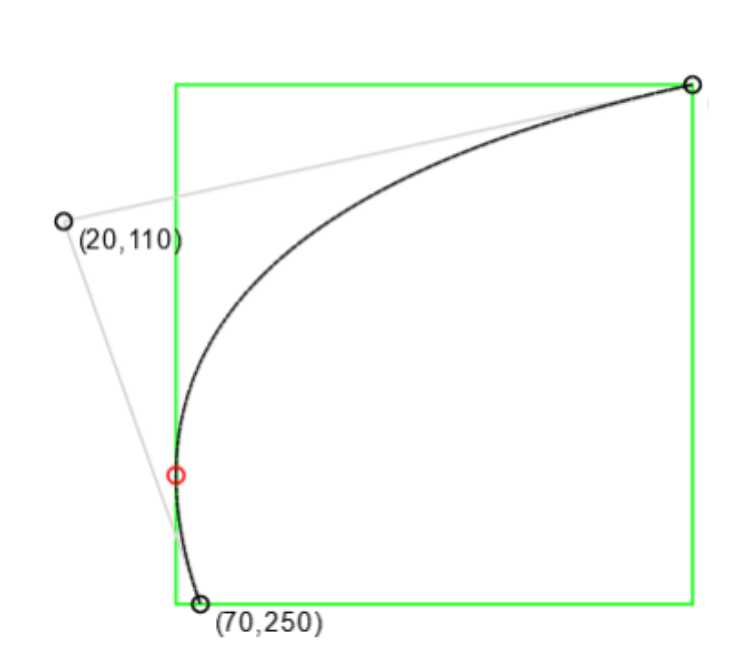
In many game development projects, there might be times when developers need to deal with bezier curve intersections. Curve intersections are potentially computationally expensive. So, they want to estimate a box surrounding the curve. Such that the curve intersection algorithm only needs to be run when it is absolutely necessary. An example bounding box for a quadratic bezier curve is below.
We know that we are using a summation of the vector of fixed points to create our curve. We can break that vector into its individual components. If we assume that we are working with a 2D bezier curve, we can break that vector into an x component and a y component.
We want to find the points on the curve that are most likely to define the bounding box. These are the points that tend to be the farthest out in any direction.
Again, getting the derivative of the vector is key. We can rephrase the problem as searching for extrema. Potential points for our bounding box include the extrema in the x component and the extrema in the y component.
The derivative gives us the rate of change. Each extreme represents a sign change in the rate of change. So, by setting the derivative of the x component and y component to 0, we can find possible points that create our bounding box.
Not all extreme points will be used, but all of them have the potential to be on the boundary of the box. In addition, it’s important to include the fixed point of the curve. If you look at the image above, One extrema and the two fixed points define the box in which the curve lies completely.